Key concepts

• logit function
• logistic function
• perfectly separable cases
• Uses MLE, not OLS

Useful info

• There is no conjugate prior of the likelihood function in logistic regression.
• Logistic regression is more accurate than naive bayes when there is more data
• inverse logit and logistic function are the same thing
• Steepest changes occur at the middle
  • change in probability scale differs depending on where the change is made in logit scale. see below.

logit <- function(p) {
  log(p/(1-p))
}
logit(0.5)

## [1] 0

logit(0.6)

## [1] 0.4054651

logit(0.9)

## [1] 2.197225

logit(0.93)

## [1] 2.586689

Interpretation

The difficulty of interpretation occurs due to the non linearity. “The curve of the logistic function requires us to choose where to evaluate changes”.

• a unit increase in \(x_i\) corresponds to a unit increase in logit(y). Now this is difficult to wrap your had around. So what you can do is convert it into probability scale by choosing two values near the mean, compute corresponding probabilities for the two values, and compute the difference.
• You can look at the derivative at that mean, to mean “change in P(y_i = 1) per small unit of change in y”.
• Divide by 4 rule
  • Derivative of the logistic function is maximized when \(\alpha + \betax = 0\), this corresponds to \(\beta/4\)(the maximum difference in P(y=1) corresponding to a unit difference in x): ( A difference of 1 in explanatory variable corresponds to no more than an b/4 difference in the probability). Gives you an upper bound.

Assumptions

• outcome y are independent given the probabilities.

Evaluation

• deviance

History

• Logistic regression was developed by statistician David Cox in 1958

Issues

• No close form solution exists because of the existence of transcendental equation in log likelihood. Use IRLS(Iteratively Re-Weighted Least Squares).
• bad things happen when data points are linearly separable
  • infinite MLE exists.
  • Solution:
    • Add regularization to your objective function, which penalizes your weight vector for getting too large.
      
    • This is essentialing act of adding a prior. zero-mean Guassian with covariance \(\frac{1}{2\lambda} I\)

Tips

• Try to center variables, especially when fitting interactions

Logistic functions

• \(x_0\) = the x-value of the sigmoid’s midpoint,
• \(L\) = the curve’s maximum value, and
• \(k\) = the steepness of the curve.

x0 <- 0  # mid point
L <- 1 # max value
k <- 1 # steepnesss

x <- seq(-6,6,by = 0.1)
f <- L/(1+exp(-k*(x-x0)))


plot(x,f)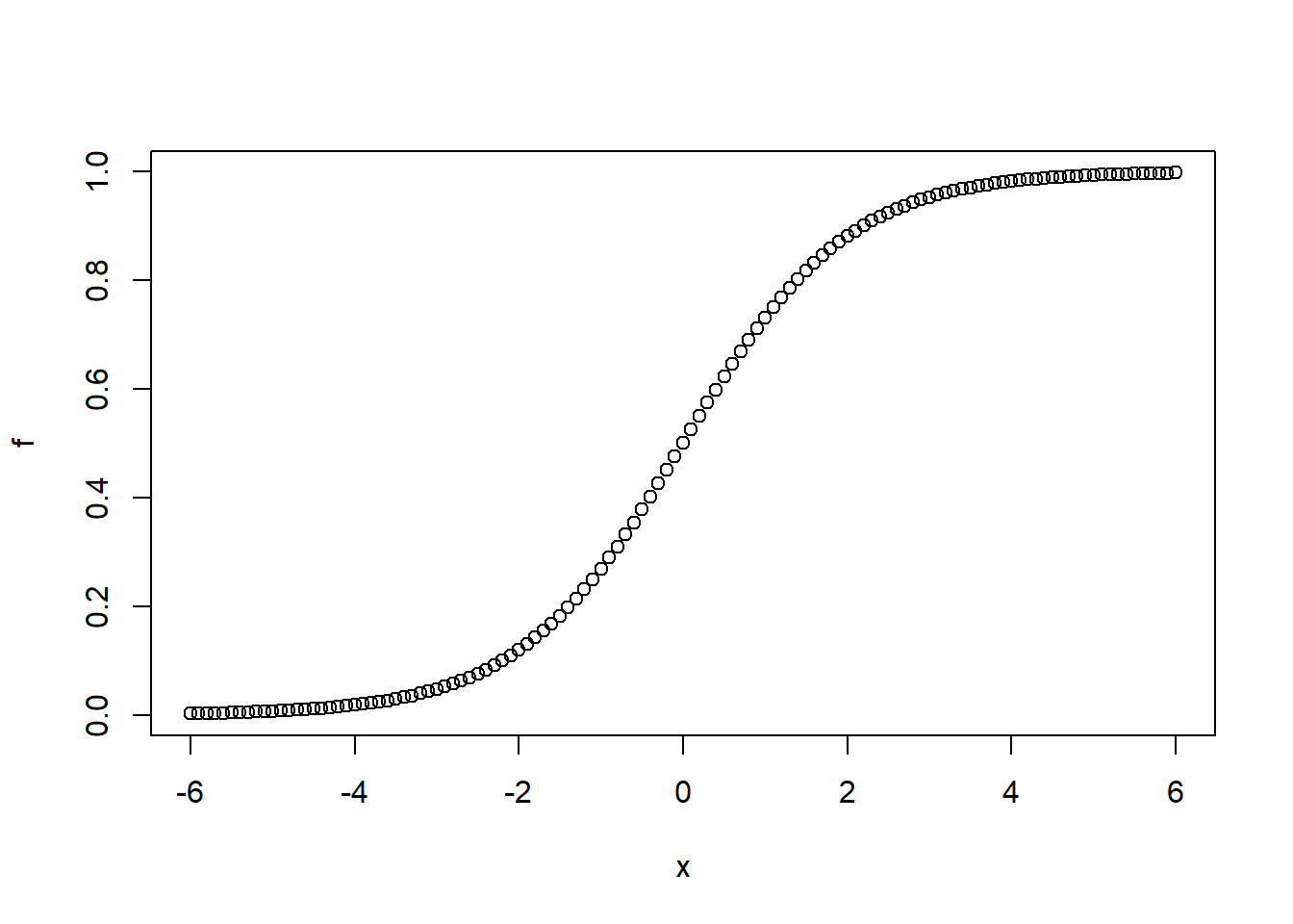

# Deviance The deviance of a model fitted by maximum likelihood is (twice) the difference between its log likelihood and the maximum log likelihood for a saturated model, i.e., a model with one parameter per observation.

Relationship to Linear Discriminant Analysis(LDA)

• LDA is a generative model
• LDA doesn’t suffer from Separation Problem.
• For small data, LDA is more stable
• LDA is better when the number of classes is greater than 2.
• The only difference between the two approaches lies in the fact that in LR(\(\beta_0\) and \(\beta_1\)) are estimated using maximum likelihood, whereas \(c_0\) and \(c_1\) are computed using the estimated mean and variance from a normal distribution.
• LDA can be computed computed directly directly from the data without without using search algorithm.
  • For a single predictor model, use a plugin estimate for \(\mu\), \(\sigma^2\), and \(pi_k\) .
• QDA is a extension of LDA where you fit separate covariance matrices for each class.
• Why does it matter whether or not we assume that the K classes share a common covariance matrix? In other words, why would one prefer LDA to QDA, or vice-versa? The answer lies in the bias-variance trade-off.
  • Consequently, LDA is a much less flexible classifier than QDA, and so has substantially lower variance. This can potentially lead to improved prediction performance. But there is a trade-off: if LDA’s assumption that the K classes share a common covariance matrix is badly off, then LDA can suffer from high bias.
• You can use MASS::lda or MASS::qda in R